Using advanced formulas and functions to enhance the functionality of financial models
Excel Functions for Finance
Here are the top 10 most important functions and formulas you need to know, plain and simple. Follow this guide and you’ll be ready to tackle any financial problems in Excel. It should be noted that while each of these formulas and functions are useful independently, they can also be used in combinations that make them even more powerful. We will point out these combinations wherever possible.
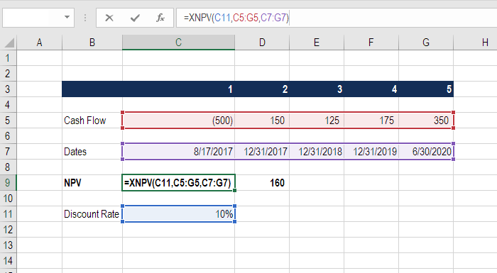
XNPV
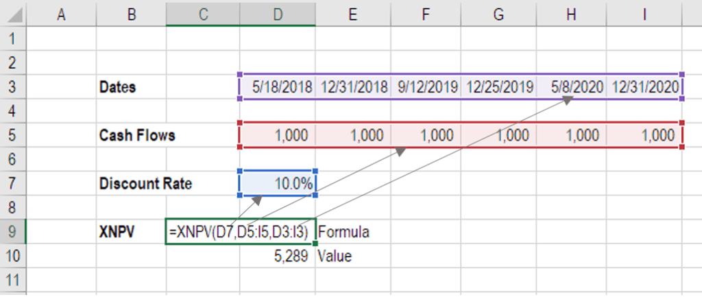
Formula: =XNPV(discount_rate, cash_flows, dates)
The number one formula in Excel for finance professionals has to be XNPV. Any valuation analysis aimed at determining what a company is worth will need to determine the Net Present Value (NPV) of a series of cash flows.
Unlike the regular NPV function in Excel, XNPV takes into account specific dates for cash flows and is, therefore, much more useful and precise.
To learn more, check our free Excel Crash course.
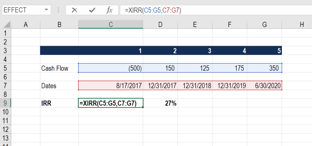
XIRR
Formula: =XIRR(cash flows, dates)
Closely related to XNPV, another important function is XIRR, which determines the internal rate of return for a series of cash flows, given specific dates.
XIRR should always be used over the regular IRR formula, as the time periods between cash flows are very unlikely to all be exactly the same.
To learn more, see our guide comparing XIRR vs IRR in Excel.
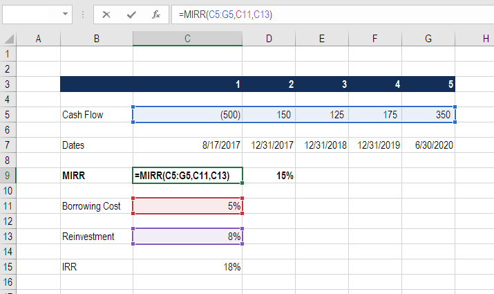
MIRR
Formula: =MIRR(cash flows, cost of borrowing, reinvestment rate)
Here is another variation of the internal rate of return that’s very important for finance professionals. The M stands for Modified, and this formula is particularly useful if the cash from one investment is invested in a different investment.
For example, imagine if the cash flow from a private business is then invested in government bonds.
If the business is high returning and produces an 18% IRR, but the cash along the way is reinvested in a bond at only 8%, the combined IRR will be much lower than 18% (it will be 15%, as shown in the example below).
Below is an Example of MIRR in action.
PMT
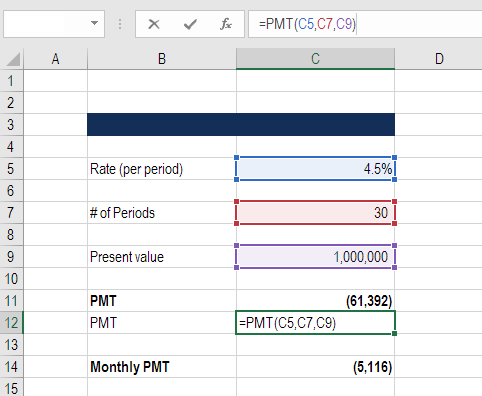
Formula: =PMT(rate, number of periods, present value)
This is a very common function in Excel for finance professionals working with real estate financial modeling. The formula is most easily thought of as a mortgage payment calculator.
Given an interest rate, and a number of time periods (years, months, etc.) and the total value of the loan (e.g., mortgage) you can easily figure out how much the payments will be.
Remember this produces the total payment, which includes both principal and interest.
See an example below that shows what the annual and monthly payments will be for a $1 million mortgage with a 30-year term and a 4.5% interest rate.
IPMT
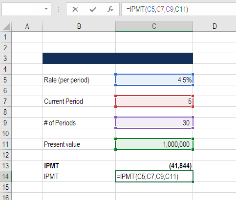
Formula: = IPMT(rate, current period #, total # of periods, present value)
IPMT calculates the interest portion of a fixed debt payment. This Excel function works very well in conjunction with the PMT function above. By separating out the interest payments in each period, we can then arrive at the principal payments in each period by taking the difference of PMT and IMPT.
In the example below, we can see that the interest payment in year 5 is $41,844 on a 30-year loan with a 4.5% interest rate.
EFFECT
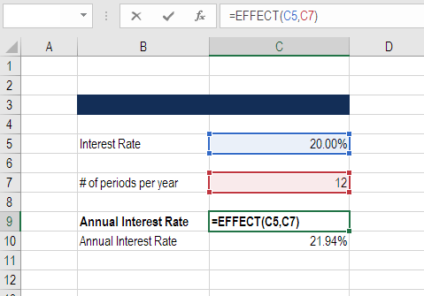
Formula: =EFFECT(interest rate, # of periods per year)
This finance function in Excel returns the effective annual interest rate for non-annual compounding. This is a very important function in Excel for finance professionals, particularly those involved with lending or borrowing.
For example, a 20.0% annual interest rate (APR) that compounds monthly is actually a 21.94% effective annual interest rate.
See a detailed example of this Excel function below.
DB
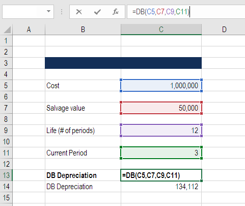
Formula: =DB(cost, salvage value, life/# of periods, current period)
This is a great Excel function for accountants and finance professionals. If you want to avoid building a large Declining Balance (DB) depreciation schedule, Excel can calculate your depreciation expense in each period with this formula.
Below is an example of how to use this formula to determine DB depreciation.
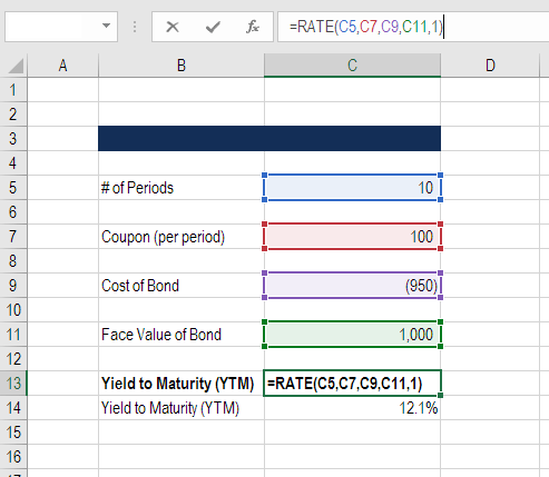
RATE
Formula: =RATE(# of periods, coupon payment per period, price of bond, face value of bond, type)
The RATE function can be used to calculate the Yield to Maturity for a security. This is useful when determining the average annual rate of return that is earned from buying a bond.
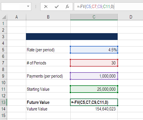
FV
Formula: =FV(rate, # of periods, payments, starting value, type)
This function is great if you want to know how much money you will have in the future, given a starting balance, regular payments, and a compounding interest rate.
In the example below, you will see what happens to $25 million if it’s grown at 4.5% annually for 30 years and receives $1 million per year in additions to the total balance. The result is $154.6 million.
To learn more, check out our Advanced Excel Formulas Course.
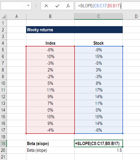
SLOPE
Formula: =SLOPE(dependent variable, independent variable)
Finance professionals often have to calculate the Beta (volatility) of a stock when performing valuation analysis and financial modeling. While you can grab a stock’s Beta from Bloomberg or from CapIQ, it’s often the best practice to build the analysis yourself in Excel.
The slope function in Excel allows you to easily calculate Beta, given the weekly returns for a stock and the index you wish to compare it to.
The example below shows exactly how to calculate beta in Excel for financial analysis.
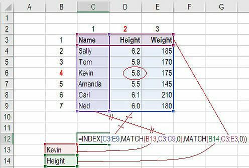
INDEX MATCH
Formula: =INDEX(C3:E9,MATCH(B13,C3:C9,0),MATCH(B14,C3:E3,0))
This is an advanced alternative to the VLOOKUP or HLOOKUP formulas (which have several drawbacks and limitations). INDEX MATCH[1] is a powerful combination of Excel formulas that will take your financial analysis and financial modeling to the next level.
INDEX[2] returns the value of a cell in a table based on the column and row number.
MATCH[3] returns the position of a cell in a row or column.
Here is an example of the INDEX and MATCH formulas combined together. In this example, we look up and return a person’s height based on their name. Since name and height are both variables in the formula, we can change both of them!
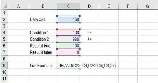
Formula: =IF(AND(C2>=C4,C2<=C5),C6,C7)
Anyone who’s spent a great deal of time doing various types of financial models knows that nested IF formulas can be a nightmare. Combining IF with the AND or the OR function can be a great way to keep formulas easier to audit and easier for other users to understand. In the example below, you will see how we used the individual functions in combination to create a more advanced formula.
OFFSET combined with SUM or AVERAGE
Formula: =SUM(B4:OFFSET(B4,0,E2-1))
The OFFSET function on its own is not particularly advanced, but when we combine it with other functions like SUM or AVERAGE we can create a pretty sophisticated formula. Suppose you want to create a dynamic function that can sum a variable number of cells. With the regular SUM formula, you are limited to a static calculation, but by adding OFFSET you can have the cell reference move around.
How it works: To make this formula work, we substitute the ending reference cell of the SUM function with the OFFSET function. This makes the formula dynamic and the cell referenced as E2 is where you can tell Excel how many consecutive cells you want to add up. Now we’ve got some advanced Excel formulas!
Below is a screenshot of this slightly more sophisticated formula in action.
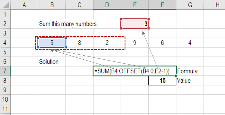
As you see, the SUM formula starts in cell B4, but it ends with a variable, which is the OFFSET formula starting at B4 and continuing by the value in E2 (“3”), minus one. This moves the end of the sum formula over 2 cells, summing 3 years of data (including the starting point). As you can see in cell F7, the sum of cells B4:D4 is 15, which is what the offset and sum formula gives us.
CHOOSE
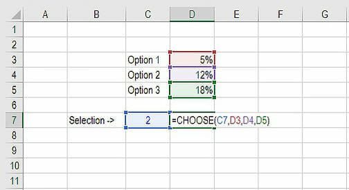
Formula: =CHOOSE(choice, option1, option2, option3)
The CHOOSE function is great for scenario analysis in financial modeling. It allows you to pick between a specific number of options, and return the “choice” that you’ve selected. For example, imagine you have three different assumptions for revenue growth next year: 5%, 12%, and 18%. Using the CHOOSE formula you can return 12% if you tell Excel you want choice #2.
Read more about scenario analysis in Excel.
To see a video demonstration, check out our Advanced Excel Formulas Course.
XNPV and XIRR
Formula: =XNPV(discount rate, cash flows, dates)
If you’re an analyst working in investment banking, equity research, financial planning & analysis (FP&A), or any other area of corporate finance that requires discounting cash flows, then these formulas are a lifesaver!
Simply put, XNPV and XIRR allow you to apply specific dates to each individual cash flow that’s being discounted. The problem with Excel’s basic NPV and IRR formulas is that they assume the time periods between cash flow are equal. Routinely, as an analyst, you’ll have situations where cash flows are not timed evenly, and this formula is how you fix that.
For a more detailed breakdown, see our free IRR vs XIRR formulas guide as well as our XNPV guide.
SUMIF and COUNTIF
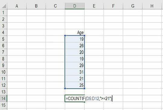
Formula: =COUNTIF(D5:D12,”>=21″)
These two advanced formulas are great uses of conditional functions. SUMIF adds all cells that meet certain criteria, and COUNTIF counts all cells that meet certain criteria. For example, imagine you want to count all cells that are greater than or equal to 21 (the legal drinking age in the U.S.) to find out how many bottles of champagne you need for a client event. You can use COUNTIF as an advanced solution, as shown in the screenshot below.
In our advanced Excel course, we break these formulas down in even more detail.
PMT and IPMT
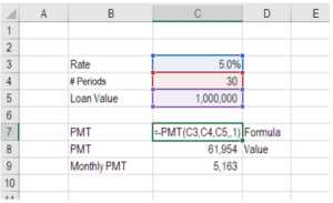
Formula: =PMT(interest rate, # of periods, present value)
If you work in commercial banking, real estate, FP&A or any financial analyst position that deals with debt schedules, you’ll want to understand these two detailed formulas.
The PMT formula gives you the value of equal payments over the life of a loan. You can use it in conjunction with IPMT (which tells you the interest payments for the same type of loan), then separate principal and interest payments.
Here is an example of how to use the PMT function to get the monthly mortgage payment for a $1 million mortgage at 5% for 30 years.
LEN and TRIM
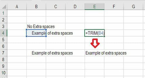
Formulas: =LEN(text) and =TRIM(text)
The above formulas are a little less common, but certainly very sophisticated ones. They are great for financial analysts who need to organize and manipulate large amounts of data. Unfortunately, the data we get is not always perfectly organized and sometimes, there can be issues like extra spaces at the beginning or end of cells.
The LEN formula returns a given text string as the number of characters, which is useful when you want to count how many characters there are in some text.
In the example below, you can see how the TRIM formula cleans up the Excel data.
CONCATENATE
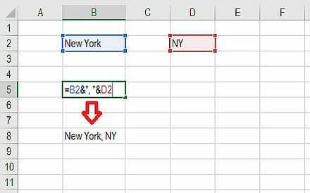
Formula: =A1&” more text”
Concatenate is not really a function on its own – it’s just an innovative way of joining information from different cells and making worksheets more dynamic. This is a very powerful tool for financial analysts performing financial modeling (see our free financial modeling guide to learn more).
In the example below, you can see how the text “New York” plus “, “ is joined with “NY” to create “New York, NY”. This allows you to create dynamic headers and labels in worksheets. Now, instead of updating cell B8 directly, you can update cells B2 and D2 independently. With a large data set, this is a valuable skill to have at your disposal.
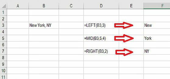
10. CELL, LEFT, MID and RIGHT functions
These advanced Excel functions can be combined to create some very advanced and complex formulas to use. The CELL function can return a variety of information about the contents of a cell (such as its name, location, row, column, and more). The LEFT function can return text from the beginning of a cell (left to right), MID returns text from any start point of the cell (left to right), and RIGHT returns text from the end of the cell (right to left).
Below is an illustration of the three formulas in action.